Example workflow using FUSE

library(methFuse)

Reading in data

We start by reading in the data, which consist of the tables K0 and K1. Both have CpG sites as rows and samples as columns, and

K0 contains the unmethylated counts
K1 contains the methylated counts

This is a dummy data set consisting of manipulated counts of the 100 000 first CpG sites in chromosome 20.

k0_file <- system.file("examples/k0.tsv.gz", package = "methFuse")
k1_file <- system.file("examples/k1.tsv.gz", package = "methFuse")

K0 <- read.table(k0_file, header = TRUE)
K1 <- read.table(k1_file, header = TRUE)

head(K0)

##             Sample1 Sample2 Sample3 Sample4 Sample5 Sample6 Sample7 Sample8
## chr20.60008       0       6       0       0       0       0       0       0
## chr20.60009       0       0       9       0      17       0      17       0
## chr20.60119      21       0       0      22       0      21       0       3
## chr20.60120      17       0       0      21      16      19       0       0
## chr20.60578       0      16       0       8       5       0       0      19
## chr20.60579       0      13      17       0      10       0       0      11
##             Sample9 Sample10 Sample11 Sample12 Sample13 Sample14 Sample15
## chr20.60008       0       17       18        0        7        0        0
## chr20.60009      17        7        1       19        3       16        0
## chr20.60119       0       21        6        0        0       17       16
## chr20.60120       0        0       19        0        0        0       11
## chr20.60578       0        4        0        4       15        0        0
## chr20.60579       0        2       20        0        0       16        6
##             Sample16 Sample17 Sample18 Sample19 Sample20
## chr20.60008       17       13       17       21        0
## chr20.60009       16       10        0       16        0
## chr20.60119        3        2       15        9        0
## chr20.60120        0        0        5       18        0
## chr20.60578       19        0        0       22        0
## chr20.60579        0        2        0        0        9

Apply FUSE as a pipeline

The whole FUSE pipeline can be applied using the function ‘fuse.segment()’. It performs the following steps:

clustering
cutting clustering tree optimally
summarizing segments

The function takes as input the count matrices K0 and K1 and the chromosome and position information for each CpG site, and outputs a summary table and a data frame with betas.

segment_result <- fuse.segment(
  as.matrix(K0),
  as.matrix(K1),
  chr = sub("\\..*$", "", rownames(K0)),
  pos = as.integer(sub("^.*\\.", "", rownames(K0))),
  method = "BIC"
)

head(segment_result$summary)

##       Segment   Chr Start   End CpGs Length      Beta Coherent
## 1 chr20.60008 chr20 60008 61140   17   1133 0.8378468    FALSE
## 2 chr20.61141 chr20 61141 61817   12    677 0.8450438    FALSE
## 3 chr20.61818 chr20 61818 63862   18   2045 0.8514536    FALSE
## 4 chr20.63863 chr20 63863 64424   13    562 0.8565943    FALSE
## 5 chr20.64609 chr20 64609 64728    6    120 0.6418476    FALSE
## 6 chr20.64778 chr20 64778 65365    6    588 0.1449167    FALSE

head(segment_result$betas_per_segment)

##               Sample1   Sample2   Sample3    Sample4   Sample5    Sample6
## chr20.60008 0.7331288 0.7795786 0.8133333 0.84156977 0.7853659 0.81250000
## chr20.61141 0.8740920 0.7928571 0.8174157 0.86084906 0.8803612 0.89154013
## chr20.61818 0.8943894 0.8278388 0.7691083 0.89508197 0.8259587 0.82819383
## chr20.63863 0.8560748 0.8793103 0.8287154 0.87633262 0.7705628 0.81779661
## chr20.64609 0.5810056 0.7909605 0.5865385 0.63636364 0.6150943 0.71794872
## chr20.64778 0.2077922 0.1000000 0.2321429 0.02764977 0.0000000 0.07692308
##               Sample7    Sample8   Sample9   Sample10  Sample11  Sample12
## chr20.60008 0.8653251 0.89727127 0.9042357 0.81441718 0.7964169 0.8934911
## chr20.61141 0.9152120 0.94017094 0.7426326 0.85650224 0.7752294 0.7946429
## chr20.61818 0.8787313 0.77701544 0.8374291 0.83053691 0.8900145 0.8762376
## chr20.63863 0.8160622 0.77941176 0.8909513 0.74315789 0.8958333 0.9621749
## chr20.64609 0.6912442 0.69565217 0.7898551 0.51933702 0.6346154 0.6311111
## chr20.64778 0.2844037 0.05769231 0.1984733 0.08024691 0.1188811 0.1530612
##              Sample13   Sample14  Sample15  Sample16  Sample17   Sample18
## chr20.60008 0.8477930 0.85780526 0.8138848 0.8699187 0.8298755 0.89660743
## chr20.61141 0.9192140 0.91549296 0.8333333 0.8463357 0.8592965 0.78795812
## chr20.61818 0.8681481 0.81139756 0.8013468 0.8629283 0.8820059 0.93140244
## chr20.63863 0.8687783 0.83193277 0.8916479 0.9232614 0.8540434 0.80167015
## chr20.64609 0.5294118 0.66666667 0.6567164 0.4928910 0.6908213 0.65024631
## chr20.64778 0.1682692 0.05462185 0.2631579 0.1298077 0.2117117 0.05952381
##              Sample19  Sample20
## chr20.60008 0.7971014 0.9366603
## chr20.61141 0.7953092 0.8556034
## chr20.61818 0.9240924 0.8153619
## chr20.63863 0.9120172 0.9628713
## chr20.64609 0.6808511 0.6701031
## chr20.64778 0.2166667 0.2110092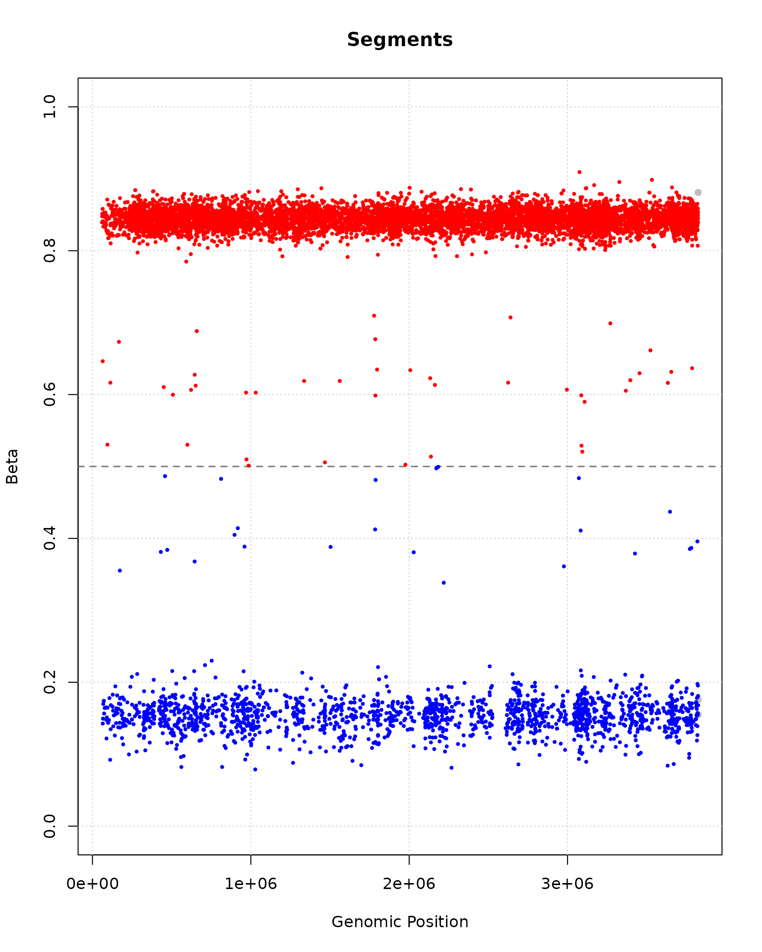

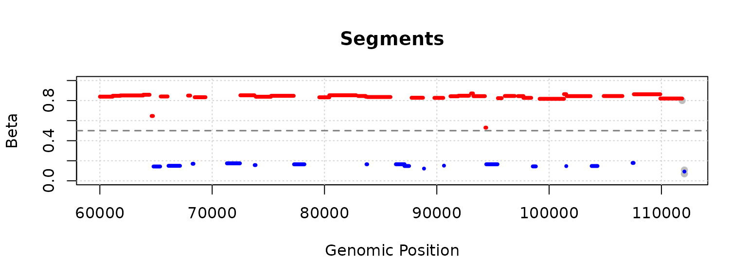
plot(segment_result, segments_to_plot = 1:nrow(segment_result$summary))

plot(segment_result, segments_to_plot = 50:60)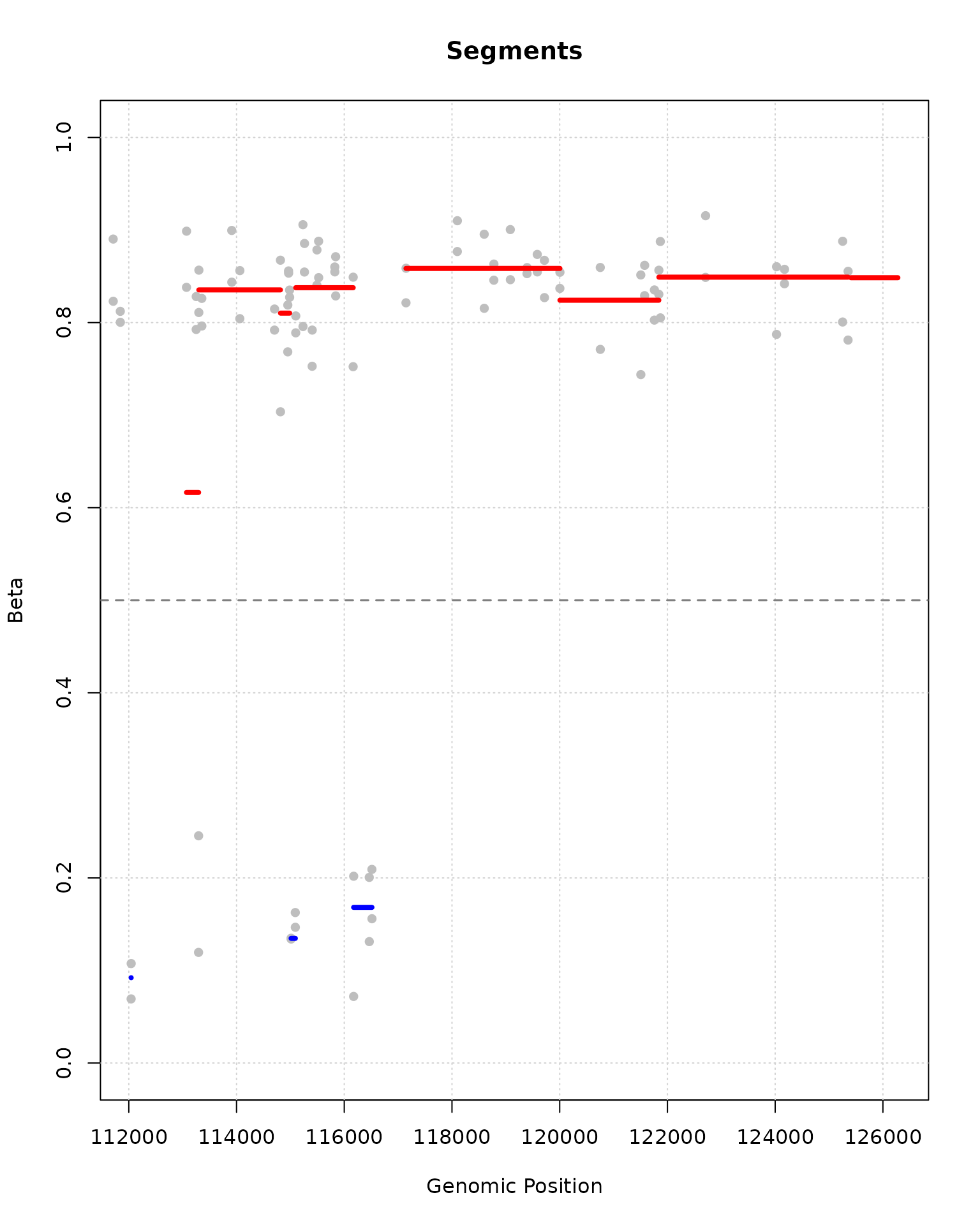

Using BSseq or methrix

The ‘fuse.segment()’ function accepts as input also a BSseq or a methrix object.

library(bsseq)

set.seed(1)
M <- matrix(c(sample(0:10, 1000, TRUE),
              sample(50:60, 1000, TRUE),
              sample(0:10, 1000, TRUE),
              sample(20:30, 1000, TRUE))
            , nrow = 1000, byrow = T)
Cov <- M + matrix(sample(50:60, 4000, TRUE), nrow = 1000)
  
  
bs <- BSseq(
    chr = rep("chr1", 1000),
    pos = seq_len(1000),
    M = M,
    Cov = Cov,
    sampleNames = colnames(M)
  )

res <- fuse.segment(bs)
head(res$summary)

##    Segment  Chr Start  End CpGs Length       Beta Coherent
## 1   chr1.1 chr1     1  250  250    250 0.08344157    FALSE
## 2 chr1.251 chr1   251  500  250    250 0.50035855     TRUE
## 3 chr1.501 chr1   501  750  250    250 0.08405464    FALSE
## 4 chr1.751 chr1   751 1000  250    250 0.31483887     TRUE

library(methrix)

data(methrix_data, package = "methrix")

res <- fuse.segment(methrix_data)
head(res$summary)

##          Segment   Chr    Start      End CpGs   Length       Beta Coherent
## 1 chr21.27866423 chr21 27866423 47286854   82 19420432 0.09796720     TRUE
## 2 chr21.47286962 chr21 47286962 47517454  118   230493 0.16972343     TRUE
## 3 chr21.47517456 chr21 47517456 47520741  211     3286 0.05453577     TRUE
## 4 chr21.47536415 chr21 47536415 47540455  129     4041 0.11761019     TRUE
## 5 chr22.45083239 chr22 45083239 49007398  203  3924160 0.13991860     TRUE

Apply FUSE through separate steps

If the intermediate outputs of the method are relevant, then the pipeline can also be applied by calling each of the functions ‘fuse.cluster()’, ‘number.of.clusters()’, ‘fuse.cut.tree()’, and ‘fuse.summary()’ separately.

1. Cluster

In the first step, ‘fuse.cluster()’ is applied on the count matrices. This performs a hierarchical clustering of closest neighbors, and outputs a clustering tree of class ‘hclust’.

tree <- fuse.cluster(as.matrix(K0), 
                     as.matrix(K1),
                     chr = sub("\\..*$", "", rownames(K0)), 
                     pos = as.integer(sub("^.*\\.", "", rownames(K0))))
names(tree)

## [1] "merge"       "height"      "order"       "labels"      "call"       
## [6] "method"      "dist.method"

head(tree$merge)

##        [,1]   [,2]
## [1,] -45579 -45580
## [2,] -57737 -57738
## [3,] -46190 -46191
## [4,] -49658 -49659
## [5,] -23937 -23938
## [6,] -41560 -41561

head(tree$height)

## [1] 10.65993 23.28925 35.99633 48.57419 65.21045 82.47522

The clustering tree contains the following elements:

‘merge’: the labels of the merged points
‘height’: The total log-likelihood for forming this merge
‘order’: Same order as original, since clustering is done in 1D
‘labels’: Labels of form ‘chr.pos’
‘call’: ‘fuse.cluster(K0, K1)’
‘method’: ‘fuse’
‘dist.method’: ‘fuse’

2. Cutting the tree

In order to cut the clustering tree, the optimal number of segments needs to be calculated. For this we have the function ‘number.of.clusters()’, which performs model selection by minimizing either the Bayesian Information Criterion (BIC, default), or the Akaike Information Criterion (AIC).

optimal_num_of_segments <- number.of.clusters(tree, ncol(K0), 'BIC')
optimal_num_of_segments

## [1] 9030

The tree can then be cut using ‘fuse.cut.tree()’, (or ‘cutree’ from package ‘stats’).

segments <- fuse.cut.tree(tree, optimal_num_of_segments)
head(segments, 100)

##   [1] 1 1 1 1 1 1 1 1 1 1 1 1 1 1 1 1 1 2 2 2 2 2 2 2 2 2 2 2 2 3 3 3 3 3 3 3 3
##  [38] 3 3 3 3 3 3 3 3 3 3 4 4 4 4 4 4 4 4 4 4 4 4 4 5 5 5 5 5 5 6 6 6 6 6 6 7 7
##  [75] 7 7 7 7 7 7 7 7 7 7 8 8 8 8 8 8 8 8 8 8 8 8 8 8 9 9

3. Summarizing segments

The segments can be summarized in a table with the function ‘fuse.summary()’.

result <- fuse.summary(as.matrix(K0), 
                       as.matrix(K1), 
                       chr = sub("\\..*$", "", rownames(K0)), 
                       pos = as.numeric(sub("^.*\\.", "", rownames(K0))), 
                       segments)

head(result$summary)

##       Segment   Chr Start   End CpGs Length      Beta Coherent
## 1 chr20.60008 chr20 60008 61140   17   1133 0.8378468    FALSE
## 2 chr20.61141 chr20 61141 61817   12    677 0.8450438    FALSE
## 3 chr20.61818 chr20 61818 63862   18   2045 0.8514536    FALSE
## 4 chr20.63863 chr20 63863 64424   13    562 0.8565943    FALSE
## 5 chr20.64609 chr20 64609 64728    6    120 0.6418476    FALSE
## 6 chr20.64778 chr20 64778 65365    6    588 0.1449167    FALSE

head(result$betas_per_segment)

##               Sample1   Sample2   Sample3    Sample4   Sample5    Sample6
## chr20.60008 0.7331288 0.7795786 0.8133333 0.84156977 0.7853659 0.81250000
## chr20.61141 0.8740920 0.7928571 0.8174157 0.86084906 0.8803612 0.89154013
## chr20.61818 0.8943894 0.8278388 0.7691083 0.89508197 0.8259587 0.82819383
## chr20.63863 0.8560748 0.8793103 0.8287154 0.87633262 0.7705628 0.81779661
## chr20.64609 0.5810056 0.7909605 0.5865385 0.63636364 0.6150943 0.71794872
## chr20.64778 0.2077922 0.1000000 0.2321429 0.02764977 0.0000000 0.07692308
##               Sample7    Sample8   Sample9   Sample10  Sample11  Sample12
## chr20.60008 0.8653251 0.89727127 0.9042357 0.81441718 0.7964169 0.8934911
## chr20.61141 0.9152120 0.94017094 0.7426326 0.85650224 0.7752294 0.7946429
## chr20.61818 0.8787313 0.77701544 0.8374291 0.83053691 0.8900145 0.8762376
## chr20.63863 0.8160622 0.77941176 0.8909513 0.74315789 0.8958333 0.9621749
## chr20.64609 0.6912442 0.69565217 0.7898551 0.51933702 0.6346154 0.6311111
## chr20.64778 0.2844037 0.05769231 0.1984733 0.08024691 0.1188811 0.1530612
##              Sample13   Sample14  Sample15  Sample16  Sample17   Sample18
## chr20.60008 0.8477930 0.85780526 0.8138848 0.8699187 0.8298755 0.89660743
## chr20.61141 0.9192140 0.91549296 0.8333333 0.8463357 0.8592965 0.78795812
## chr20.61818 0.8681481 0.81139756 0.8013468 0.8629283 0.8820059 0.93140244
## chr20.63863 0.8687783 0.83193277 0.8916479 0.9232614 0.8540434 0.80167015
## chr20.64609 0.5294118 0.66666667 0.6567164 0.4928910 0.6908213 0.65024631
## chr20.64778 0.1682692 0.05462185 0.2631579 0.1298077 0.2117117 0.05952381
##              Sample19  Sample20
## chr20.60008 0.7971014 0.9366603
## chr20.61141 0.7953092 0.8556034
## chr20.61818 0.9240924 0.8153619
## chr20.63863 0.9120172 0.9628713
## chr20.64609 0.6808511 0.6701031
## chr20.64778 0.2166667 0.2110092

Verification

The outputs are identical.

identical(segment_result$summary, result$summary)

## [1] TRUE

identical(segment_result$betas_per_segment, result$betas_per_segment)

## [1] TRUE

Plotting

Let’s visualize a small piece of the result:

plot(result, segments_to_plot = 1:50)

Susanna Holmstrom

2026-02-05